
Relaxed Barrier Functions (RBFs): Soft Constraint and Penalty Function
Rendered from robotics_notes/mpc/constraint/rbf/rbf.md.
Contents
- Constraint Margin
- Penalty Function
- Figure
- Fine-tuning
- Stronger Constraint Recipe
- Common Symptoms
- Code Implementation
- Reference literature for RBFs
This note describes the relaxed barrier functions (RBFs) penalty with self-collision constraint handling as an example.
In this repo, RBF means a relaxed logarithmic barrier penalty [1] applied as a soft state inequality constraint.
Constraint Margin
For each configured collision pair, compute the signed clearance margin
where:
- \(d_i(q)\) is the current distance for collision pair \(i\).
- \(d_{\min}\) is
selfCollision.minimumDistance. - The constraint is satisfied when \(h_i(q) \ge 0\).
The RBF self-collision cost is
So every configured pair contributes a penalty.
The runtime hard stop is separate: it checks the minimum distance over all pairs and falls back to hold mode if that minimum is below selfCollision.hardStopDistance.
Penalty Function
The relaxed barrier for a scalar inequality \(h \ge 0\) is given as
The quadratic extension makes the penalty finite and smooth when the constraint is violated. It matches the logarithmic branch in value, first derivative, and second derivative at \(h=\delta\).
The derivatives used by the solver are
and
At the boundary \(h=0\):
This is the main tuning fact: decreasing \(\delta\) makes the penalty much stiffer near and inside the boundary.
Figure
The figures in this section are generated by /rbf/assets/plot_rbf.py.
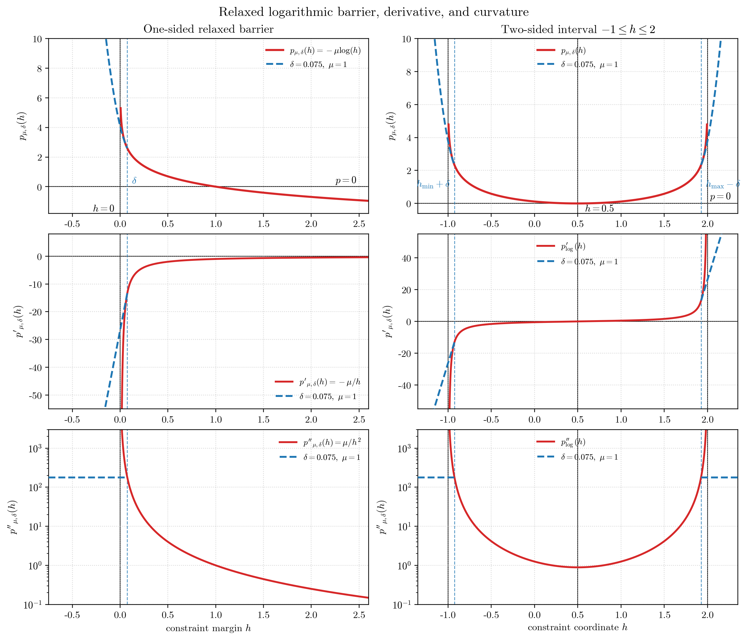
The first figure compares the unrelaxed logarithmic barrier against one relaxed barrier with \(\delta=0.5\) and \(\mu=1\). The top row shows the penalty value, the middle row shows the first derivative, and the bottom row shows the curvature. The dashed blue vertical guide lines mark the quadratic-extension switch points.
The left column shows the one-sided relaxed barrier. The right column shows a two-sided interval example built from two one-sided barriers:
This is the same idea used for pairwise self-collision: each distance margin is a one-sided inequality.
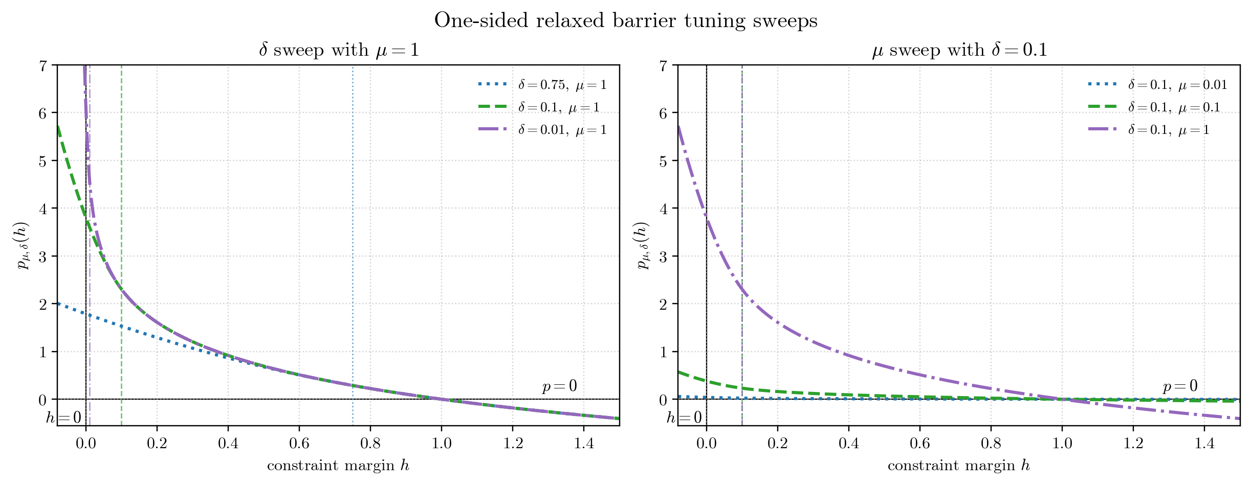
The second figure isolates the two main tuning effects with one-sided relaxed barrier penalty curves and no unrelaxed log reference. The left plot changes \(\delta\) while holding \(\mu=1\). The right plot changes \(\mu\) while holding \(\delta=0.1\). This makes the roles separate: \(\mu\) changes the penalty scale, while \(\delta\) changes where the quadratic extension begins and how stiff the violation region becomes.
Fine-tuning
Use these knobs in this order.
minimumDistance
minimumDistance changes the constraint margin itself:
Increasing minimumDistance makes avoidance start earlier because the same physical distance produces a smaller margin. If the robot reacts too late while still feasible, first increase minimumDistance before making the barrier very stiff.
mu
mu scales the penalty, gradient, and curvature linearly:
Increase mu when the optimizer treats collision avoidance as too weak relative to tracking cost. Decrease it when the robot pushes away too aggressively or tracking becomes unnecessarily biased.
Practical sweep:
delta
delta controls where the logarithmic branch switches into the quadratic relaxation. For \(h > \delta\), delta has no effect. For \(h \le \delta\), the boundary stiffness is
Smaller delta makes the penalty sharper near the limit and during violation. Larger delta makes it smoother and easier for the optimizer numerically, but also less strict near the boundary.
Practical sweep:
Avoid making delta tiny while also making mu large unless the solver still converges reliably. The local curvature grows as \(\mu/\delta^2\).
Stronger Constraint Recipe
A reasonable starting point for stronger self-collision avoidance is:
# Example constraint yaml config in ocs2 mpc
selfCollision:
  activate: true
  minimumDistance: 0.05
  hardStopDistance: 0.01
  implementation: rbf
  mu: 1.0e-2
  delta: 1.0e-4
Then tune one thing at a time:
- If avoidance starts too late:
minimumDistance\(\nearrow\). - If avoidance starts early enough but loses against tracking:
mu\(\nearrow\). - If it only fails very close to the boundary:
delta\(\searrow\). - If solve quality becomes unstable:
delta\(\nearrow\) ormu\(\searrow\).
Common Symptoms
If the robot still enters the safety distance:
minimumDistancemay be too small for the horizon and velocity.mumay be too weak relative to tracking weights.deltamay be too large, making the boundary too soft.- The horizon may be too short for the dynamics to avoid collision.
- Runtime torque, velocity, or acceleration limits may prevent the planned avoidance motion.
If the robot avoids collision but drifts away from useful poses:
mumay be too large.minimumDistancemay be larger than needed.- This RBF penalty has nonzero gradient even when the constraint is feasible. If you need zero penalty away from the boundary, use a hinge/AL style penalty instead of RBF.
Code Implementation
The OCS2 penalty implementation is in:
The code implements:
getValue()as the piecewise relaxed barrier.getDerivative()as \(p'_{\mu,\delta}(h)\).getSecondDerivative()as \(p''_{\mu,\delta}(h)\).
The self-collision margin is computed in OCS2 Pinocchio self-collision as:
Relevant files:
ocs2_pinocchio/ocs2_self_collision/src/SelfCollision.cppocs2_pinocchio/ocs2_self_collision/src/SelfCollisionCppAd.cpp.
The dynamics MPC wrapper creates the self-collision constraint and attaches the RBF penalty here:
The relevant branch is:
if (settings.implementation == "rbf") {
  problem.stateSoftConstraintPtr->add(
    "selfCollision",
    std::make_unique<ocs2::StateSoftConstraint>(
      std::move(constraint),
      std::make_unique<ocs2::RelaxedBarrierPenalty>(
        ocs2::RelaxedBarrierPenalty::Config{settings.mu, settings.delta})));
  return;
}
Both inverse dynamics and forward dynamics MPC pass the same settings into this shared helper:
The generated parameters are declared in: